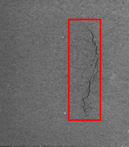
When I sell our visual quality inspection systems, I am often asked at a very early stage of the project how accurate the defect detection is. Typically, we need a Proof of Concept with a first Machine Learning (ML) model to answer this question. And the answer to the question is expressed in the form of performance metrics. This blog post gives some background on the meaning of the performance metrics we offer when doing object detection, with some examples from crack detection in the steel production:

Image 1: Image of a crack and a bounding box when using object detection – preML GmbH

For the following, it is sufficient to understand that the output of an easy ML classification model is a prediction based on patterns or relationships learned by the model from a training data set. In our example, the training dataset would consist of the images of the parts on which we have marked (annotated) cracks. In addition to the training dataset, there is usually a second dataset, the test dataset, with the same type of data and annotations. The performance of an ML model is determined by comparing its predictions on the unseen test dataset with the annotations, in our example, whether the quality department would say it is a crack or not.

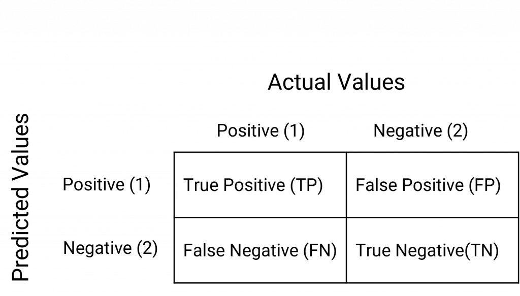
Here it is where it starts getting complicated. In the easiest ML models, we will have at least to consider four types of outputs. All cases when the model correctly predicted positive (TP), all cases where the model predicted correctly negative (TN), all cases when the model predicted positive, but it was actually negative (FP) and all cases when the model predicted negative, but it was actually positive (FN). This is known as “Confusion Matrix” as well.

Image 2: Confusion Matrix

There are many different metrics out here, but we typically would present you four metrics for an object detection model, precision, recall, AP@50 and AP@50-95:

Precision: Precision is a measure of how accurate the positive predictions made by a model are. In the context of crack detection, precision would be the ratio of correctly detected cracks to all the instances predicted as cracks. In other words, it tells us how many of the predicted cracks are actually true positives.

For example, let’s say your crack detection model predicts that there are 10 cracks in a steel plate, but upon manual inspection, only 7 of them are actual cracks. In this case, the precision would be 7/10 or 0.7, which means 70% of the predicted cracks were true positives.

Recall: Recall, also known as sensitivity or true positive rate, measures how well a model captures all the positive instances. In crack detection, recall would be the ratio of correctly detected cracks to all the actual cracks present in the steel plate. It shows how many of the actual cracks were successfully detected.

For instance, if there are 15 actual cracks in a steel plate and your model detects 10 of them, the recall would be 10/15 or approximately 0.67, which means the model captured about 67% of the actual cracks.

Precision-Recall Trade-Off: It is important to understand that no ML-algorithms performs categorical decisions on its own. Instead, they output a likelihood or “confidence” in a classification. We use percentages to communicate the confidence. For example, we say, according to the model an image contains a crack with 85% confidence. In practice, we set a threshold to perform a categorical decision based on the confidence value. For example, we could determine that all detections with a confidence higher than 50% are considered as cracks. By changing this decision threshold, we either improve precision or recall while harming the other.

Understanding the concepts of precision and recall forms the foundation for evaluating more comprehensive metrics that are crucial in the context of object detection. As mentioned, with object detection we identify and localizing multiple objects (such as a crack) in an image or video frame.

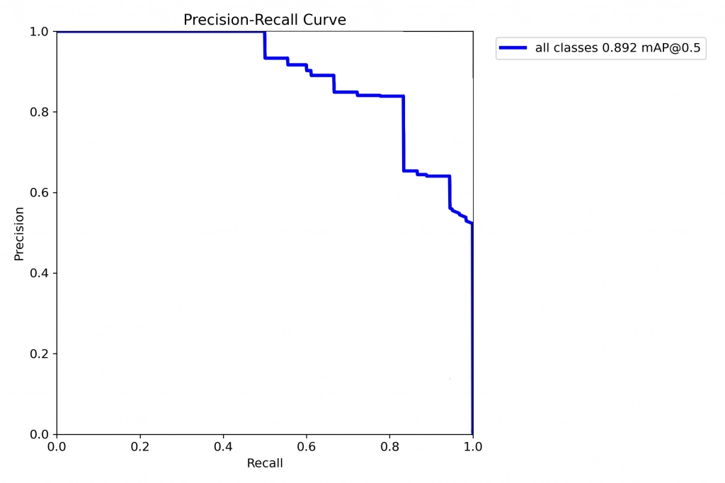
Average Precision (AP): By calculating precision and recall for all confidences between 0% and 100% we can create a plot showing all possible precision-recall combinations. To get a metric summarizing precision and recall, we can simply calculate the area under this curve. This value is called Average Precision (AP).

Image 2: Precision-Recall curve for a object detection algorithm – preML GmbH

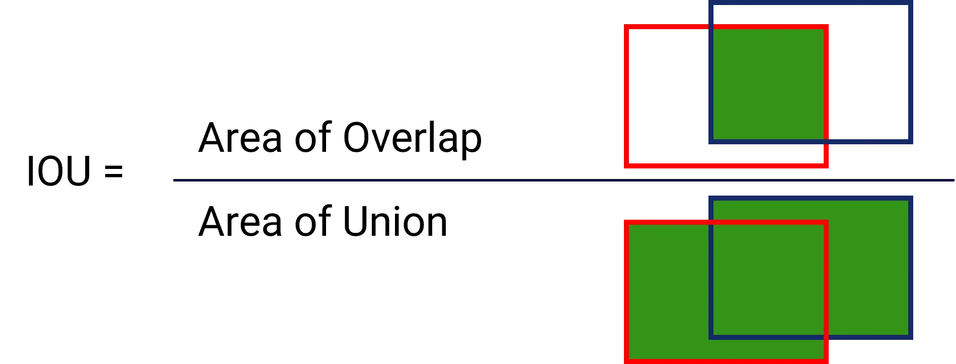
Image 3: IoU visualisation. Red Boxes are Ground Truth vs. Blue Boxes the Prediction of a Object Detection Model – preML GmbH

AP@50: Average Precision at 50 (mAP@50) is a metric often used in object detection tasks and we typically mention this value as the one to be aware of in a Proof of Concept phase for example. It considers precision and recall over a range of confidence thresholds and calculates the average precision. The “@50” indicates that the boxes have to have at least 50% overlap (see IoU) to be considered a true positive.

In the context of crack detection, this metric would evaluate how well your model performs at different confidence levels in predicting cracks. It averages the precision-recall curve at a confidence threshold of 50%.

AP@50-95: Similar to AP@50, AP@50-95 calculates the average precision, but it takes into account a range of IoU thresholds from 50% to 95%. This metric provides a stricter evaluation of the model’s performance by looking at higher IoU thresholds.

Remember, in practical applications, a good model should strike a balance between high precision and high recall. A model with high precision but low recall might miss some important cracks, while a model with high recall but low precision might produce many false positives. We use average precision to create a combined metric of precision and recall. The choice of which metric to emphasize depends on the specific requirements of the task and the potential consequences of missing detections or false alarms in the production.

Remember as well, the performance metrics interact with the data and annotation quality. If the model is very good, it will find defects which the annotator might have missed in the annotation phase.

I guess that’s it for the moment!

Looking forward for feedback to this article

Cheers!

David & Lucas

Contact us at contact@preml.io or connect with me on LinkedIn